


“Don’t leave money on the table.” Some version of that line comes up again and again in meetings where simulation is presented. Most systems are complex enough that finding the right solution is far easier said than done. To land on the exact combination of conditions that delivers the best possible performance, you have to examine many scenarios.
Every situation can call for some change to your model, and the sheer number of parameters and combinations can produce thousands, even hundreds of thousands, of possible experiments.

That leaves you facing an impractical task, and real improvements go unrealized simply because there was never enough time to experiment. “Great presentation. Are you sure you’ve found the best solution for our business?”
With ProcessModel the task becomes far easier. PM Optimizer, which is built into ProcessModel, automates the work of trying settings, running the model, and comparing the results. You tell it which settings it may change and what you want to improve, and it searches for the combination that does best. Set a goal of the highest throughput with the fewest resources and the lowest work in progress, and PM Optimizer runs the experiments, changes the settings, compares the output, and shows you the best configurations, all while you get on with something else.
When to use process optimization
When should you optimize? You need it once the number of choices exceeds the number of experiments you are willing to run by hand. A natural starting point is around 15 experiments. Past that, set the model up for optimization. It takes only a few minutes to configure, and you can do other things while the computer runs the experiments. When the numbers get large, let the optimizer run while you go to lunch or head home for the night, and the best solution will be waiting when you return.
How many experiments might be needed
It depends on the number of factors and the number of choices for each. To find the count, multiply the options for one choice by the options for the next. If there are 3 job functions and the staffing for each can vary by 5 (say, from 15 to 20), the number of possibilities is 125.
Think of it this way: 5 choices for the first factor, and for each of those, 5 choices for the second, which is 5 x 5 = 25. For each of those 25 combinations, 5 choices for the third, and so on, giving 125. It is easy to see how fast this gets out of hand. With just 6 factors at five choices each, you are at nearly 16,000 experiments. Add two more factors and the count exceeds 390,000.
Design of experiments
In a complex system, design of experiments is used to limit the number of trials to save time and money. That means some experiments are never run, because of an arbitrary decision not to try those combinations. Rather than cut possibilities artificially, why not let the computer eliminate trials based on the responses it actually sees? That is what simulation optimization does. It performs a smart design of experiments and learns as it goes.
PM Optimizer does this with its Smart Optimizer. It spreads a first batch of experiments across the whole space, learns which areas look promising, and works those, a batch at a time. In an optimization with over 400,000 possible experiments, a search like that can find a strong configuration after only a small fraction of them. You set a run budget, anywhere from 20 runs to 1,000, and it stops when the budget is spent or when better results stop coming. That is automated design of experiments at work.
There is another catch. Classic design of experiments was not really built to handle a range of possibilities for each factor (such as 15 to 20). Use a range and the number of experiments grows dramatically, and you are back to sifting through huge result sets to decide which is best, doing the analysis yourself. In a complex system that can mean hundreds of hours poring over data to find the best result.
How to do optimization
It is really not that hard.
- Prepare a validated model
- Open PM Optimizer
- Choose the settings to adjust
- Set the goals for optimization
- Optimize
- Plug the optimization values into the model

Prepare a validated model
This article is not about validating models, so I will keep this short, but do not optimize unless the model is validated. Optimizing an unvalidated model is a gamble, with a high chance the outcome is wrong. A few simple checks go a long way: watch the animation to confirm the model performs every intended function, make sure the input data is correct, test all distributions, export the model data and check each time value, time unit, capacity, queue size, and move time (I use a red pen to tick off each entry), and compare both the overall output and the critical parts against real data from company systems. Building a model of the as-is system this way is exactly how you gain confidence in its predictive power before you start making changes.
Open PM Optimizer
To make the steps easy to follow, we will use a very simple model, though the same procedure applies to complex ones.
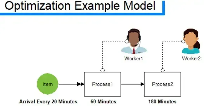
In this model, items arrive every 20 minutes. The first activity, Process1, takes 60 minutes, and the second, Process2, takes 180 minutes. The goal is to maximize throughput with the minimum resources. You could work out in your head that three workers are needed at the first activity and nine at the second. You would not normally simulate a model whose answer you already know, but this simple example makes the steps clear.
Because Worker1 is assigned to Process1, the capacity of that activity has to be large enough to hold the assigned workers. Without that, it is as if you have plenty of resources but no workspace for them. Set the capacity of Process1 to 4 and the capacity of Process2 to 10, the most workers you will try at each, so the search is free to move the workers. Do this before you open PM Optimizer, because the model cannot be edited while it is open.
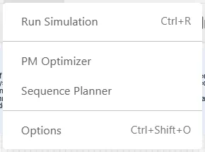
With a validated model in hand, open PM Optimizer from the Simulate menu, alongside Run Simulation and Option, or from the toolbar button just after Simulate. It opens in its own window over your model, and it always measures your model as it stands today, so you have a Baseline to compare the winner against.
Choose the settings to adjust
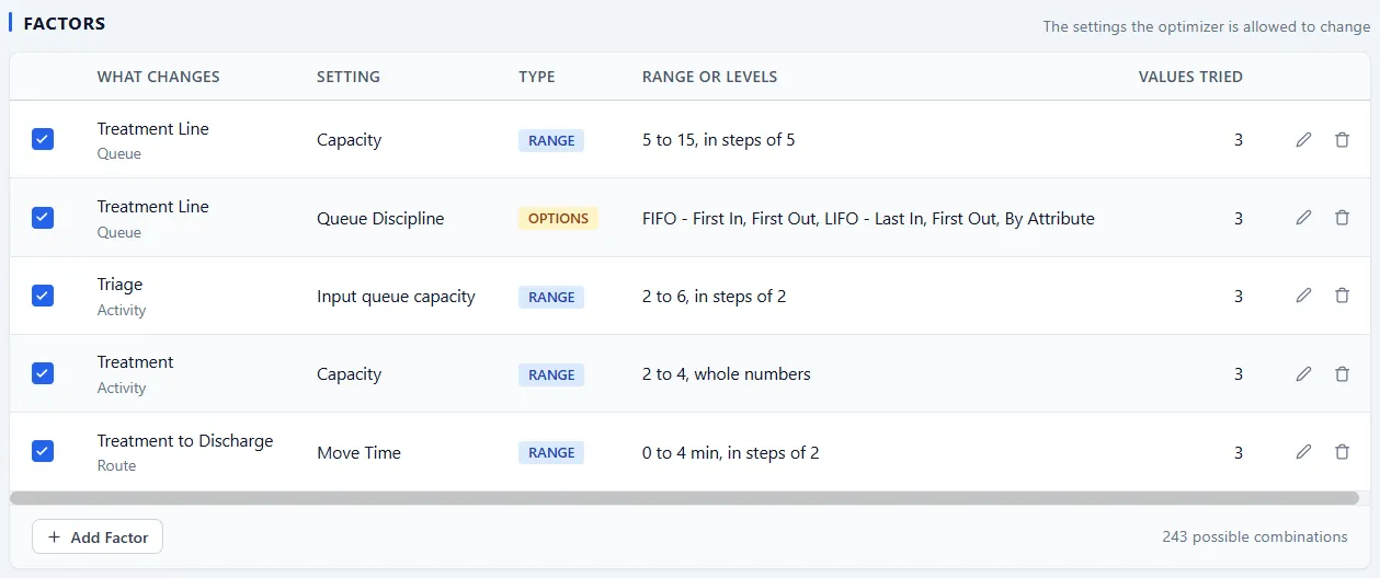
On the Define step, the first thing to fill in is the factors table. A factor is a setting you allow PM Optimizer to change while it searches, and Add Factor opens a picker that lists everything in your model you can change, grouped by the kind of object. You choose the real setting on the real object, so there is nothing to prepare in the model first. Here is the factors table from a triage model.
In our example the settings to change are the number of workers. Choose the card for Worker1, pick its Quantity, choose Use a range, and enter a minimum of 1 and a maximum of 4. Save Factor adds it to the table. Do the same for Worker2, with a minimum of 7 and a maximum of 10. Even though we know the answer, I will pretend I do not and let the search roam the whole range.
Setting the range matters for two reasons. First, limiting the range reduces the number of experiments, so the search finds a result faster. Second, the real system may have physical limits that cannot be exceeded. If floor space restricts you to three machines, letting the count vary from 1 to 5 is pointless unless building changes are on the table; the conservative range would be 1 to 3.
Set the goals for optimization
Next, tell PM Optimizer what best means. You do that by choosing the results to measure, which it calls responses: throughput, average time in system, cost per entity, work in process and more. Every response carries a goal: Lower is better for something you want less of, such as time or cost, and Higher is better for something you want more of, such as throughput. One response wears the Primary badge and leads the search. Here are the responses of the same triage model.
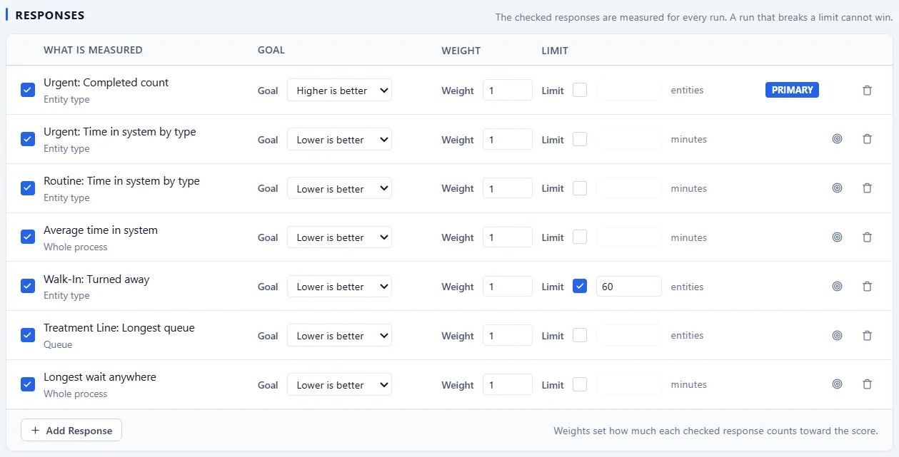
PM Optimizer only knows what you tell it through the responses. If they measure just throughput, that is all it improves. Leave out the cost of the workers and it assumes you do not care how many you use. When more than one response counts, give each a weight so they combine into a single score. A higher weight pulls the search harder toward that response.
In our example we maximize the items processed while minimizing the number of resources. Add Throughput as a response with the goal Higher is better. To count the workers, give each worker an hourly cost and add Total run cost as a response with the goal Lower is better. Give both the same weight and they count equally; raise one and the search leans toward it.
You can also put a limit on a response, a floor or a ceiling the result must respect. A configuration that breaks a limit still runs and is still reported, but it cannot win.
Optimize
With the settings and goals in place, choose how PM Optimizer explores the combinations. The design is the trade-off between how thorough the search is and how long it takes.
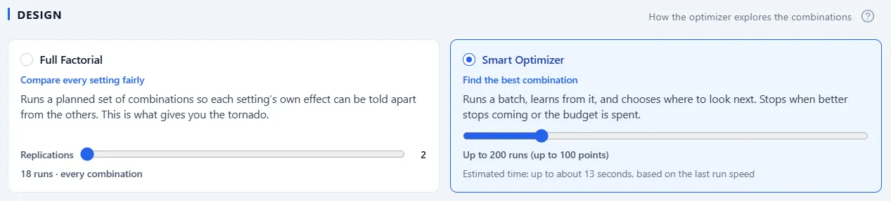
The Smart Optimizer is the default, and the right choice when your aim is to find the best configuration. It runs a batch, learns from it, and chooses where to look next. You set its run budget, from 20 runs to 1,000, and it stops when the budget is spent or when better results stop coming. A model with variability gives a slightly different answer every run, so it gives every configuration a quick pass first, then re-runs the leaders together until the group stops changing. That puts the precision where the decision is. Full Factorial suits a few settings when you want the complete picture: it runs a planned set of combinations so each setting’s own effect can be told apart from the others.
The bar along the bottom of the Define step does the arithmetic before you commit, with the number of runs and, once PM Optimizer has timed a run in your session, about how long they will take. When you are ready, choose Save & Run Experiment, which saves the experiment and starts it. The Run step then shows the work as it goes, with a best-so-far line that climbs as configurations finish and a Stop button if you have seen enough.
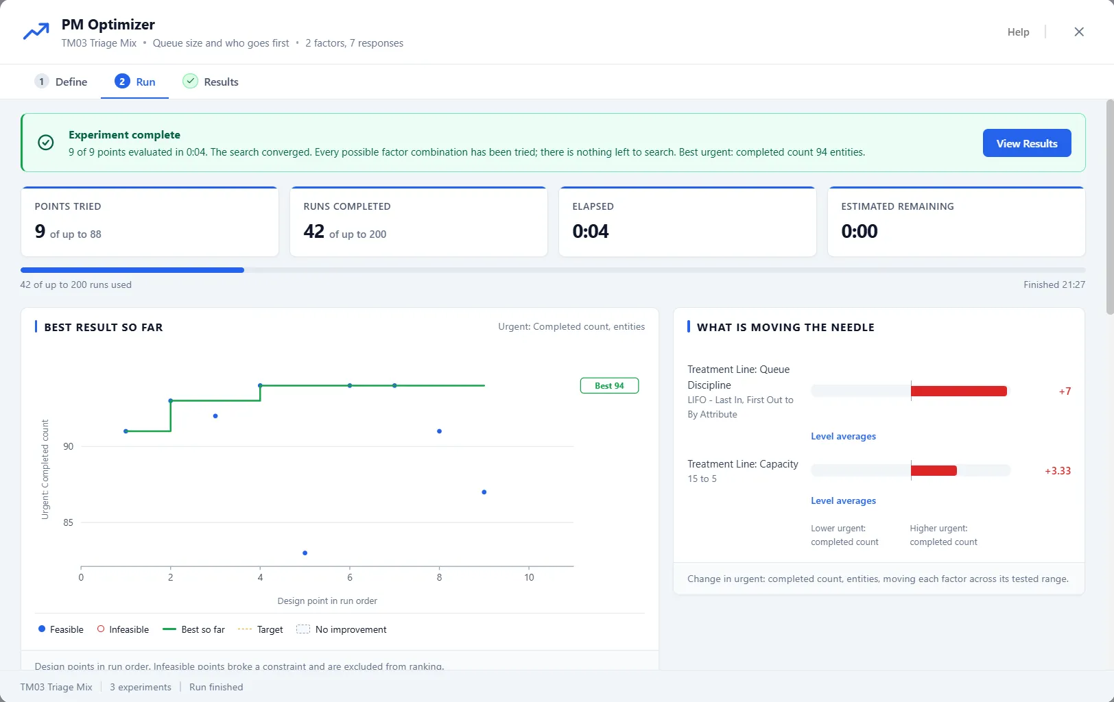
There are many capabilities this tutorial will not cover. The whole area of pre-analysis to determine warm-up length and the number of replications is covered in the Basics II training class.
Plug the optimization values into the model
When the run finishes, PM Optimizer opens the Results step. A band at the top says what the run can honestly claim: when one configuration stands out, it names it and says how much better it is, and when the leaders cannot be told apart, it says how many are tied for best. Below it, every configuration is ranked, with the settings it used and the value of each response, and a Baseline row leads the table: your model today, unchanged.
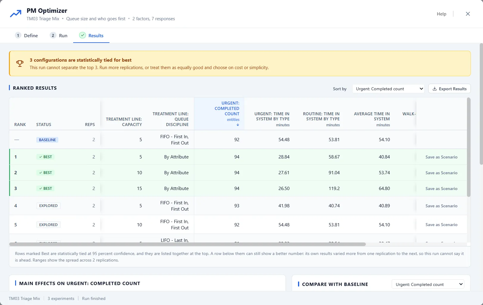
In a model as small as ours you can check the table against the answer you worked out by hand. The Baseline row is today’s model, with 3 workers at the first activity and 9 at the second, and no listed row is exactly 3 and 9. Compare the Baseline against the rows tied for best: they reach the same throughput as the Baseline, which is the answer you worked out. When several rows are tied for best, you are free to choose among them on cost or simplicity.
The optimization should not be the final run of the model. When you have chosen, select Save as Scenario on that row. It copies the configuration into your model as an ordinary scenario, enabled and ready to run, and nothing the experiment did changed your model or your saved results. Take the time to run the model with the new scenario and read the report. That gives you added assurance the model is working correctly with the new values, and a chance to spot other improvement areas that were not part of your goals.
PM Optimizer searches using feedback from your own simulation model, and it ranks every configuration it tried, so you get not just a single optimized solution but a ranked list of strong alternatives.
If you want to stop leaving money on the table, see what ProcessModel and PM Optimizer can do or explore plans and pricing.